Dataset Overview

The dataset is accessible for download [1] and is meticulously curated by Muhammad Talha Awan under the CC0 License [2]. It contains vital statistics regarding global sugar consumption.

Technical Focus: Cartopy Shapereader

To obtain shapefiles for all countries, utilize the shapereader functionalities to download and store the data locally:

import cartopy.io.shapereader as shpreader

shapename = 'admin_0_countries'

countries_shp = shpreader.natural_earth(resolution='10m',

category='cultural', name=shapename)

The downloaded shapefiles can be iterated over. We define a function to retrieve all countries that fall within specified sugar consumption boundaries:

def country_sugar_consumption(lower, upper):

country_list = []

for record in shpreader.Reader(countries_shp).records():

country = record.attributes['NAME']

consumption = df.query('(Name == @country) & (Action == "consumption")')['2018/19']

if len(consumption) == 0:

continue

consumption = float(consumption.values[0].replace(',',''))

if consumption > lower and consumption <= upper:

country_list.append(record.geometry)

return country_list

To visualize the colored polygons on the plot, we implement the following code:

fig = plt.figure(figsize=(7, 5))

ax = fig.add_subplot(projection=ccrs.EckertIII())

# Add all countries

ax.add_geometries(shpreader.Reader(countries_shp).geometries(),

ccrs.PlateCarree(),

facecolor='C7', alpha=0.1

)

# All countries with sugar consumption in bottom 25%

ax.add_geometries(

country_sugar_consumption(0, 1919),

ccrs.PlateCarree(),

facecolor='C0', edgecolor='C7')

# All countries with sugar consumption in 25% - 50%

ax.add_geometries(

country_sugar_consumption(1919, 2519),

ccrs.PlateCarree(),

facecolor='C1', edgecolor='C7')

# All countries with sugar consumption in 50% - 75%

ax.add_geometries(

country_sugar_consumption(2519, 8827),

ccrs.PlateCarree(),

facecolor='C2', edgecolor='C7')

# All countries with sugar consumption in 75% - 100%

ax.add_geometries(

country_sugar_consumption(8827, 1e9),

ccrs.PlateCarree(),

facecolor='C3', edgecolor='C7')

# Legend items

q0 = mpatches.Rectangle((0, 0), 1, 1, facecolor='C0')

q1 = mpatches.Rectangle((0, 0), 1, 1, facecolor='C1')

q2 = mpatches.Rectangle((0, 0), 1, 1, facecolor='C2')

q3 = mpatches.Rectangle((0, 0), 1, 1, facecolor='C3')

q4 = mpatches.Rectangle((0, 0), 1, 1, facecolor='C7')

labels = ['No data', '< 25%', '25% - 50%', '50% - 75%', '> 75%']

ax.legend([q4, q0, q1, q2, q3], labels,

loc='lower left', bbox_to_anchor=(0.025, 0), fancybox=True)

What is the sugar consumption per country?

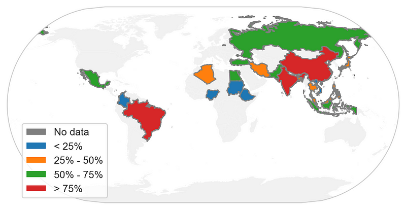
We extract data on sugar consumption per nation for the year 2018/19 from the dataset. Unfortunately, the dataset lacks unit measurements. We categorize the countries into four quantiles corresponding to their global sugar consumption levels. For countries with no data, we leave them uncolored, while the remaining countries are represented on the plot and colored based on their respective quantile. The top consumers tend to be the most populous countries, notably India, China, and Brazil.

Which countries export more sugar than they consume?

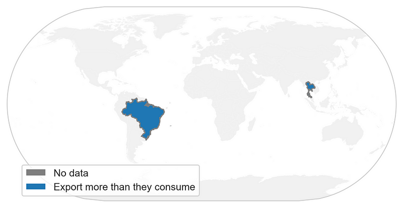
We analyze the dataset to identify countries that export more sugar than they consume. Only two nations meet this criterion: Brazil and Thailand.

Which countries have the highest growth in sugar consumption?

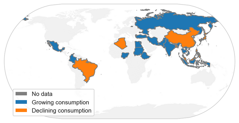
Next, we investigate which nations experienced growth in sugar consumption by comparing data from 2022 and 2018. While overall sugar consumption appears to be on the rise, several countries, including China, Japan, the Philippines, Bangladesh, and Brazil, show a decline in consumption.

Summary

In this analysis, we utilized several Python libraries:

• Pandas for data handling and manipulation
• Cartopy for visual representation

Focus Function:

All visualizations and images included were generated by the author unless otherwise specified.

Explore all previous Friday Data Story notebooks on GitHub:

If you enjoyed this data narrative, please give a clap, follow the author, and subscribe to the publication for future updates.