Understanding the Time-Dependent Schrödinger Equation

To explore the evolution of quantum mechanical particles over time, one must tackle the time-dependent Schrödinger equation. In most scenarios, computational assistance is necessary for solving this equation, as the implementation can be more complex than it initially appears. However, with the right approach, it can be accomplished succinctly in Python.

The time-dependent Schrödinger equation is expressed as follows:

Here, the Hamiltonian acts as a differential operator concerning the spatial coordinates. The standard method involves discretizing both time and spatial derivatives, but there are nuances to consider in achieving an effective solution.

To start, we discretize the time derivative using a forward difference scheme, allowing us to express it as:

In this representation, the upper index indicates the time step, defined as follows:

At this stage, we have not yet discretized the spatial variables. We can solve for the wave function at the new time step, which leads us to:

It’s important to note that we aim to express the spatial derivatives in the wave function. In principle, we could compute the new state solely by applying the operator from the previous time step. This approach is termed an explicit scheme because the new solution directly depends on the prior solution. However, this method proves ineffective as it fails to conserve the norm of the wave function. The true Schrödinger equation must maintain that the total probability of locating the particle is always one, underscoring the need for numerical schemes that uphold this principle.

An alternative approach could involve rearranging the equation to yield:

In this case, the new wave function is present on the right side of the equation. We cannot directly solve for the new state but can formulate an equation that applies to it, leading to what is known as an implicit scheme:

Typically, one would discretize the spatial variables here, converting the wave function into a vector and the Hamiltonian into a matrix. This results in a linear system of equations to solve for the new wave function. However, this scheme also does not conserve the norm, rendering it ineffective.

A viable solution lies in combining both explicit and implicit schemes, which allows us to derive the average of their outcomes:

This can also be expressed as:

By discretizing the spatial variables now, we re-establish the system of equations to solve. Remarkably, this approach preserves the norm, providing the desired outcome. This methodology is known as the Crank-Nicholson scheme.

In a different form, we can rearrange the equation to explicitly express the new wave function:

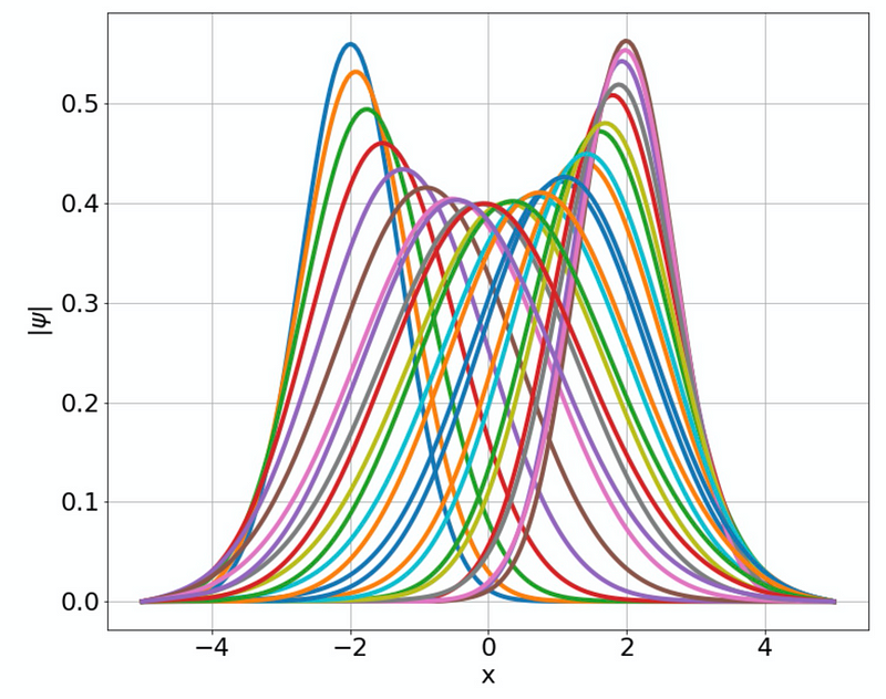
The matrix introduced here represents the discretized time propagation operator within the Crank-Nicholson framework. Let's implement this scheme in Python to model a particle oscillating in a harmonic oscillator potential: